Reasoning logic

The reasoning logic is where properties of a specification are stated and proved. Formulas of the reasoning logic appear in Theorem, Axiom, Define, CoDefine, Query, assert, and the other commands that take a formula.

Syntax

The following table summarizes the formula and term forms.

Form	Meaning
forall A B C, F	Universal quantification.
exists A B C, F	Existential quantification.
nabla a b c, F	Nominal quantification.
F1 /\ F2	Conjunction.
F1 \/ F2	Disjunction.
F1 -> F2	Implication.
true, false	Truth and falsity.
t1 = t2	Equality.
p t1 t2	An atomic reasoning-level predicate.

Specification-level provability has three forms:

• {G}: provability from the module alone.
• {L |- G}: provability from a context L of assumptions.
• {L, [F] |- G}: provability using the backchaining assumption F.

Binding has lower precedence than the connectives, so forall x, F1 -> F2 quantifies over the whole implication. Application binds tighter than the connectives.

Terms are formed from constants, variables, application, and abstraction:

t ::= c | x | t1 t2 | x\ t | f^n t

Abstraction is written with a backslash: x\ t. The type of x may be annotated: (x : tm)\ t. Application is by juxtaposition, so f x y means (f x) y. The form f^n t abbreviates n applications of f, so s^3 z means s (s (s z)).

Names and nominal constants

By convention, variables begin with an uppercase letter and constants begin with a lowercase letter. The distinction is made by binding structure, not by case: a name is a variable exactly when it is bound by a quantifier, an abstraction, or a clause head. The token _ is an anonymous variable and can be used wherever a fresh variable is needed.

The nabla quantifier introduces nominal constants, displayed as n1, n2, and so on. A nominal constant stands for a name that is distinct from all other names in scope. This is how the reasoning logic represents objects with binding without committing to a particular representation of variables.

For example, the formula

nabla x, name x

says that a fresh nominal constant satisfies name. The variable x in the binder becomes a nominal constant when the formula is used.

Typing

Every term and formula must be well typed. The reasoning logic has the following built-in types:

• o, the type of formulas in the specification logic;
• olist, an abbreviation for list o, the type of lists of o formulas;
• prop, the type of formulas in the reasoning logic.

The list type constructor is built in and is written with a postfix argument, as in list tm. The constants nil and :: are the empty list and list cons, and member is predefined at every element type. Their internal types are:

nil    : list A
::     : A -> list A -> list A
member : A -> list A -> prop

:: is infix. The type argument is inferred, so X :: nil and x :: xs work without annotations. These names cannot be redeclared.

Declaring types and constants

Kind and Type extend the reasoning signature:

Kind nat type.

Type z nat.
Type s nat -> nat.

Define lt : nat -> nat -> prop by
  lt z (s N) ;
  lt (s M) (s N) := lt M N.

The types and constants of the current specification are already available under the same names.

Type annotations

Types must be inferred, and inference sometimes needs help. A binder may be annotated:

forall (x : tm) y, ...
nabla (x : tm), ...

A group of binders may share one annotation, and annotated and unannotated binders may be mixed:

forall (x y : tm) z (u : bool), predicate x y z u.

The same form is accepted by exists and nabla. The example assumes that a type named bool has been declared.

A variable occurrence may be annotated with x:t, and an abstraction with (x : tm)\ .... Type parameters on a theorem or definition support schematic polymorphism:

Theorem append_det[A] : forall (L1 : list A) L2 L3 L3',
  ...

The type parameters are implicitly instantiated at each use. See Schematic polymorphism for schematic definitions, proofs, and explicit type instantiation.

Definitions

Define introduces an inductive predicate with a fixed set of clauses:

Define ctx : olist -> prop by
  ctx nil ;
  nabla x, ctx (of x T :: L) := ctx L.

A clause with no body is equivalent to one whose body is true. The first definition can therefore be written equivalently as

Define ctx : olist -> prop by
  ctx nil := true ;
  nabla x, ctx (of x T :: L) := ctx L.

A semicolon is allowed before the first clause, and the final period may be on a line of its own. Some authors therefore prefer to put the separator at the start of each clause:

Define ctx : olist -> prop by
; ctx nil
; nabla x, ctx (of x T :: L) := ctx L
.

Abella accepts both styles and does not enforce either one.

A definition must contain at least one clause; a Define command with no clauses between by and the final period is a syntax error. To define a predicate that holds of nothing, give it a single clause whose body is false:

Define ctx : olist -> prop by
  ctx L := false.

Case analysis on such a predicate produces no subgoals.

CoDefine introduces a co-inductive predicate, using the same clause syntax:

CoDefine sim : tm -> tm -> prop by
  sim P Q := forall A P',
    step P A P' -> exists Q', step Q A Q' /\ sim P' Q'.

nabla in definition heads

A clause head may begin with nabla x,, which binds one or more nominal constants:

Define ctx : olist -> prop by
  ctx nil ;
  nabla x, ctx (of x T :: L) := ctx L.

The nabla binder is not the same as forall. A clause is implicitly universally quantified over its free variables, but nabla introduces a fresh nominal constant that the other arguments may not depend on. Consequently, the ctx clause above can prove ctx (of E T :: L) only when E is a nominal constant that does not occur in T or L.

When such a clause is unfolded or analyzed with case, Abella introduces a fresh nominal constant and raises the existing eigenvariables when their types permit dependence on it. The Close command can rule out such dependencies for particular types; see Subordination.

The definition name uses the same idea to recognize nominal constants:

Define name : tm -> prop by
  nabla x, name x.

This definition has exactly one clause. Case analysis on name E replaces E with a fresh nominal constant; there is no case for an application or any other constructor.

Freshness is the other common use of nabla in a definition head:

Define fresh : tm -> tm -> prop by
  nabla x, fresh x Z.

Because Z is quantified outside the nabla, it cannot mention the nominal constant introduced for x. Thus fresh X Z holds exactly when X is a nominal constant that does not occur in Z. For example, fresh x (app x x) is unprovable, while fresh x c is provable when c is a constant.

Pruning is the corresponding property for lists. The following theorem says that if E x is a member of a list L that is quantified outside the nabla, then E cannot depend on x:

Theorem member_prune : forall (E : tm -> o) L, nabla (x : tm),
  member (E x) L -> exists F, E = x\ F.

Here the nabla is in the theorem statement rather than in a definition head. Since L is quantified outside the nabla, it cannot contain x. The proof is a short induction on the membership derivation:

induction on 1. intros. case H1.
  search.
  apply IH to *H2. search.

The name definition appears in examples/lambda-calculus/fcurry/fcurry.thm, the fresh definition in examples/process-calculi/session_types/sess.thm, and member_prune in both.

Stratification

A definition whose body contains an implication uses the predicates in the premise negatively. Such a definition is well behaved only if no predicate depends negatively on itself or on a predicate defined later. Abella performs a simple check for this condition. By default it prints a warning if the check fails; with --strict-stratification the same finding is an error.

The check is important for consistency. A definition that violates it may allow a proof of false. The warning should be treated as an error unless you know why the definition is safe. Inside a reasoning-level module, stratification findings are always errors; see Reasoning-level modules.

Inductive restrictions

When induction is applied, Abella records the size of the inductive argument with a restriction. The annotation * means smaller than the original, and @ means equal to the original. For example, applying induction on 1. to

============================
 forall E V T, {eval E V} -> {of E T} -> {of V T}

produces

IH : forall E V T, {eval E V}* -> {of E T} -> {of V T}
============================
 forall E V T, {eval E V}@ -> {of E T} -> {of V T}

The inductive hypothesis may be used only on an argument marked *. Case analysis on an argument marked @ produces subgoals whose new hypotheses are marked *, which makes them eligible.

Restrictions do not change the meaning of a formula. They are bookkeeping that prevents circular uses of the inductive hypothesis.

Nested induction

Repeated applications of induction produce nested restrictions. For a goal outer -> inner -> result, applying induction on 1 and then induction on 2 gives:

IH : outer* -> inner -> result
IH' : outer@ -> inner** -> result
============================
 outer@ -> inner@@ -> result

The outer hypothesis IH ignores the inner restrictions. The inner hypothesis IH' requires an outer argument marked @ or * and an inner argument marked **. The multiplicity of stars or at-signs matters: ** is smaller than * in the nested ordering.

Restrictions on the goal

backchain with an inductive hypothesis can produce a goal that carries a restriction. Such a goal is inert: it can be proved only by matching a corresponding hypothesis with search. It cannot be unfolded or used to drive further case analysis.

Co-inductive restrictions

Co-induction uses the annotations + (co-smaller) and # (co-equal). The following transition system is a small example.

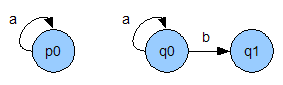
Assume the states and labels are declared and the transition relation is defined:

Kind state, label type.
Type p0, q0, q1 state.
Type a, b label.

Define step : state -> label -> state -> prop by
  step p0 a p0 ;
  step q0 a q0 ;
  step q0 b q1.

The state q0 simulates p0 if every transition of p0 can be matched by q0 and the resulting states are again related. This is a greatest fixed point, so it is stated with CoDefine:

CoDefine sim : state -> state -> prop by
  sim P Q := forall A P',
    step P A P' -> exists Q', step Q A Q' /\ sim P' Q'.

To prove sim p0 q0, start with coinduction. The proof state is:

CH : sim p0 q0 +
============================
 sim p0 q0 #

The + on the co-inductive hypothesis means that it can be used only for a goal also marked +. The # on the goal means that recursive calls produced by unfolding it will be marked +.

Unfolding the goal with unfold. gives:

CH : sim p0 q0 +
============================
 forall A P', step p0 A P' ->
   exists Q', step q0 A Q' /\ sim P' Q' +

The recursive call sim P' Q' is marked +, so search can match it with CH once the transitions have been discharged.

Duality with induction

The two kinds of restriction are dual:

• An inductively restricted hypothesis can be applied to appropriately restricted arguments. An inductively restricted goal is inert and can only match a hypothesis.
• A co-inductively restricted goal can be matched with the conclusion of a co-inductive hypothesis. A co-inductively restricted hypothesis is inert and can only match a goal.

Lemmas and mutual induction

A theorem becomes a lemma that later proofs can use by name:

Theorem my_lemma : forall X, {P X} -> {Q X}.

Theorem my_theorem : forall X, {P X} -> {R X}.
intros. apply my_lemma to H1. ...

Abella supports mutual induction on specification judgments. State the conjunction of the statements and give one induction argument per conjunct:

Theorem even_odd_nat :
  (forall X, {even X} -> {nat X}) /\
  (forall X, {odd X} -> {nat X}).

induction on 1 1. split.
  intros. case H1.
    search.
    apply IH1 to H2. search.
  intros. case H1.
    apply IH to H2. search.

The induction on 1 1 creates IH for the even statement and IH1 for the odd statement. Both hypotheses carry the same inductive restriction, so each can be used to prove the other.

To recover the individual statements, either use apply with no arguments:

Theorem even_nat : forall X, {even X} -> {nat X}.
apply even_odd_nat. search.

or use the top-level Split command:

Split even_odd_nat as even_nat, odd_nat.

Split creates both theorems directly.

Apply with unknowns

apply can leave arguments unspecified with _. Abella guesses the missing hypothesis, tries to prove it with search, and turns it into a subgoal if search fails. For example, given

H1 : ctx L
H4 : {L, of n1 T |- of (R n1) U}*
H5 : {L, of n1 T |- of (R n1) U'}
============================
 arrow T U = arrow T U'

we want to apply an inductive hypothesis that also needs ctx (of n1 T :: L). The tactic

apply IH to _ H4 H5.

lets Abella supply and discharge that argument. If the unknown cannot be solved immediately, it becomes the current subgoal, possibly with other subgoals delayed.

Unknowns are also useful with apply my_lemma. to instantiate a quantifier: the result becomes a hypothesis and the system chooses the instantiation.

Computation

The compute tactic evaluates hypotheses asynchronously. It repeatedly case-analyzes and unfolds them, stopping when a suspension guard applies or when no further progress is possible. The optional number after compute is a gas limit; the default is 1000.

A Suspend declaration names a predicate and the arguments that must remain uninstantiated for computation to stop:

Define $nat : nat -> prop by
  $nat z ;
  $nat (s X) := $nat X.

Suspend $nat X.

Theorem ten : forall X, $nat (s^10 X) -> $nat X.
intros. compute H1. search.

Here compute H1 evaluates the hypothesis until it reaches $nat X. The guard is suspended because X is still uninstantiated, so computation stops and the remaining goal can be proved by search.

compute accepts several hypotheses at once, as in compute H1 H2.. A * before a hypothesis removes it after computation, as in compute *H1.. The forms compute (all) and compute (*all) apply computation to every hypothesis. The member predicate has a built-in suspension guard on its list argument.

Forward chaining

The fchain tactic forward-chains a list of lemmas against the hypotheses in scope:

[hint:] fchain [depth] lem1 lem2 ... .

The lemmas are tried from left to right, and their immediate consequences are added as hypotheses. The optional number bounds the number of iterations and defaults to the number of lemmas. The tactic is branching: it may produce subgoals.

Type p, q, r tm -> prop.

Axiom p_q : forall X, p X -> q X.
Axiom q_r : forall X, q X -> r X.

Theorem chain : forall X, p X -> r X.
intros. fchain p_q q_r. search.

Subordination

Abella tracks which types can appear inside terms of other types. For atomic types a and b, write a <| b when a term of type a can occur inside a term of type b. Subordination is reflexive, transitive, and computed from the declared constants: if c : t1 -> ... -> tn -> a, then each ti is subordinate to a.

The relation makes dependency information explicit. If R : tm -> nat and no tm can occur inside a nat, then R must be a vacuous abstraction, and Abella can use that fact automatically.

Close fixes the subordinates of the named types:

Close tm, ty.

After this command, Abella knows that a tm cannot appear inside a ty, so it can reject or simplify terms such as T n1 where T : ty and n1 : tm. The command applies to all types subordinate to the named ones.

The types o, olist, and prop cannot be closed, because that would prevent later extensions of the specification.

Comments

A % begins a comment that runs to the end of the line. A /* ... */ comment may span lines and may be nested. Comments may appear between commands, between clauses, and between terms.